Machine Learning and Optimization in Communications

With machine learning and deep learning, artificial intelligence has entered nearly every field of engineering in the recent years. This lecture aims to teach the fundamentals of the mechanisms behind machine-/ deep learning and numerical optimizations in the context of communication engineering. Solutions to challenges of modern communication systems with the given techniques are discussed and the application of the given tools is presented.

The lecture is accompanied by a vast repository of example source code in Python using the ubiquitous PyTorch machine learning framework, so that the lecture participants can easily adapt the methods learned in the lecture to their own problems.

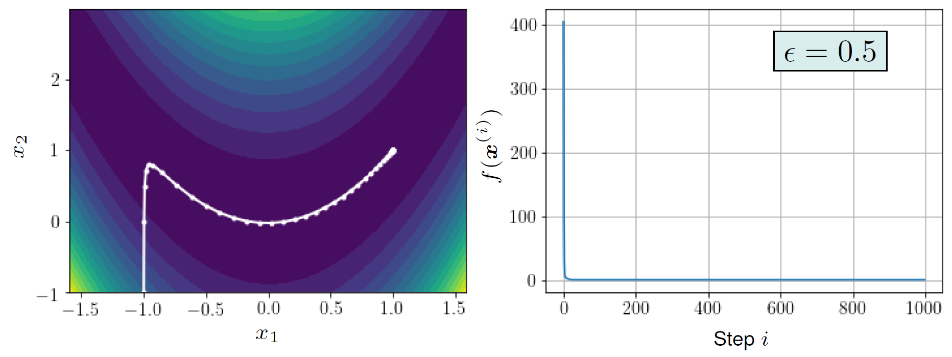
The lecture starts with a comprehensive discussion of the mathematical prerequisites needed to study machine learning and optimization. The introduction finally introduces the gradient descent algorithm, which forms the basis of nearly all modern machine learning systems. The algorithm is illustrated with many examples and interactive tools. The following figure shows an illustration of a variant of the gradient descent algorithm used to optimize a bivariate function:

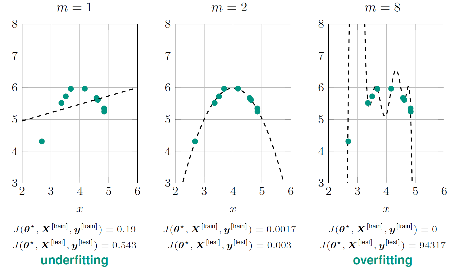
Following the introduction of the basics, we will gently introduce the basic concepts of (classical) machine learning. The concepts include different variants of learning algorithms, the concepts of training and testing, the concept of capacity and the concepts of over- und underfitting. Over- and underfitting are illustrated in the following figure using polynomial fitting. 

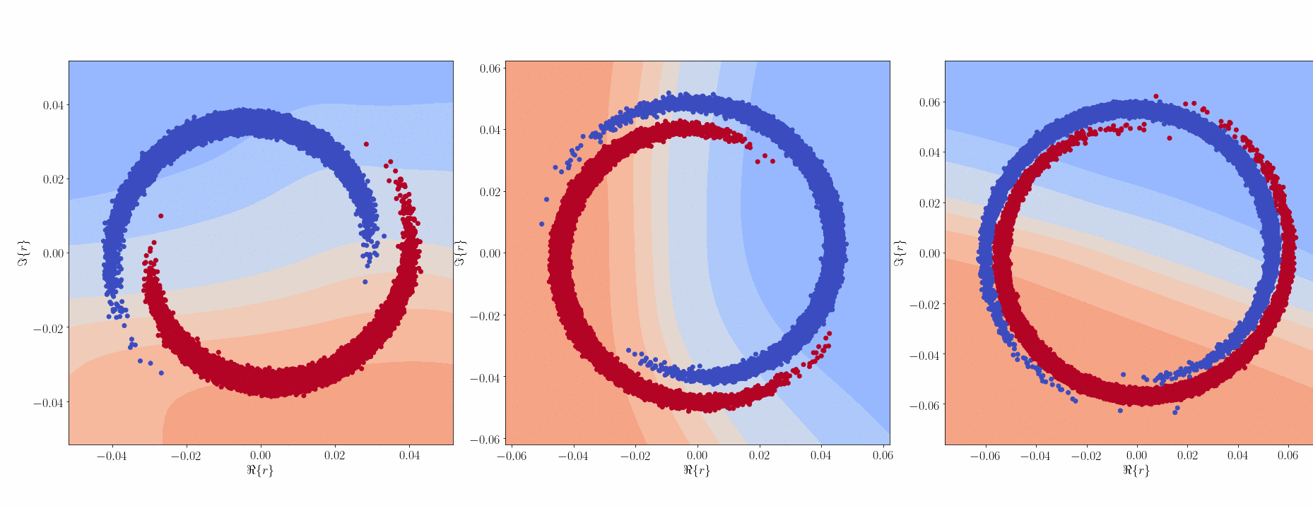
Based on our discussion on classical machine learning algorithm, we then proceed to introduce neural networks and modern deep learning systems. We introduce different variants of neural networks and show how they can be used for solving various problems in communications engineering. For instance, we show how neural networks can solve the problem of symbol detection in optical fibers, which cannot be easily solved using traditional classical communication engineering methods. The following animation shows the learned symbol detectors for a binary modulation format, which we will extend to higher-order modulation formats within the lecture.

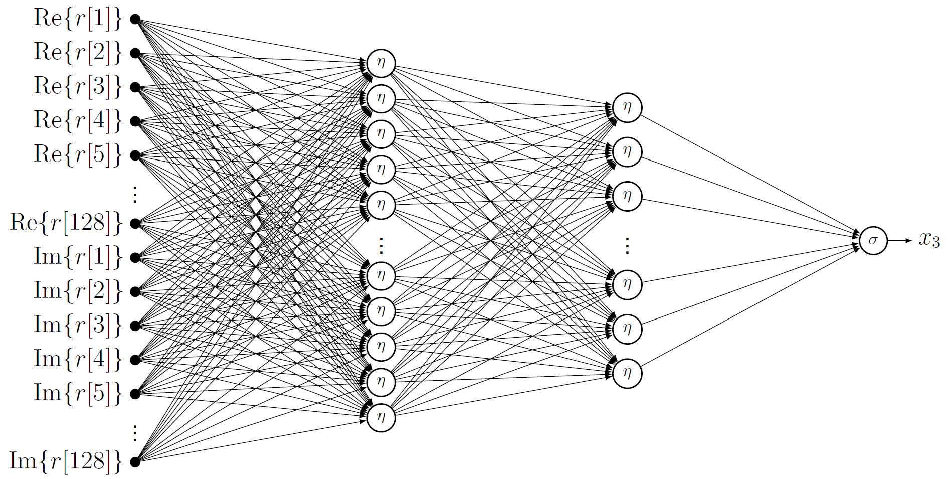
The following figure shows an example of a neural network that is used for the classification and detection of unknown modulation formats. 

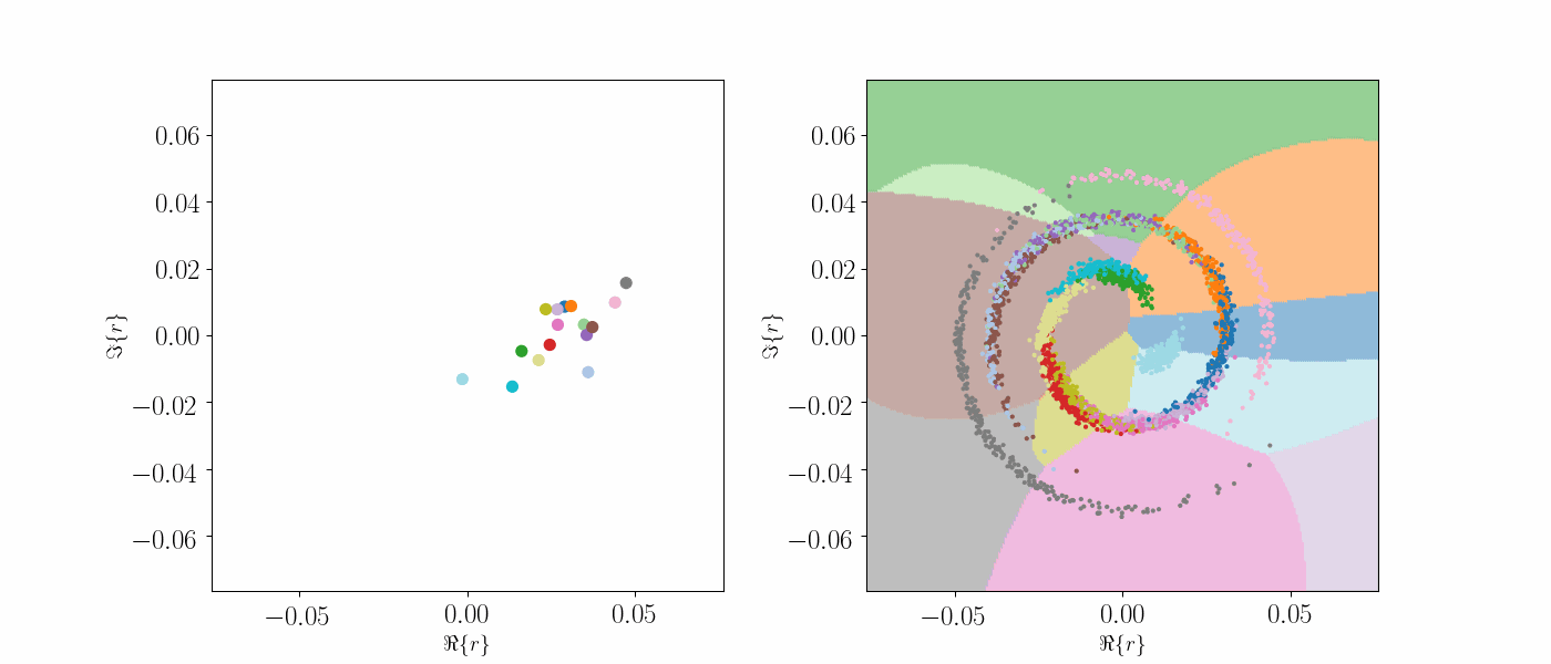
The lecture then proceeds with showing how to optimize complete transmission systems and optimize the parameters of communication systems. The following example shows the optimization of a modulation constellation for fiber-optic communications, which is a scenario that is difficult to solve with traditional methods but easy to solve with machine learning approaches:

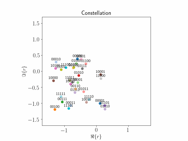
Another example is the joint optimization of modulation formats and bit assignments, which is shown in the following animation:

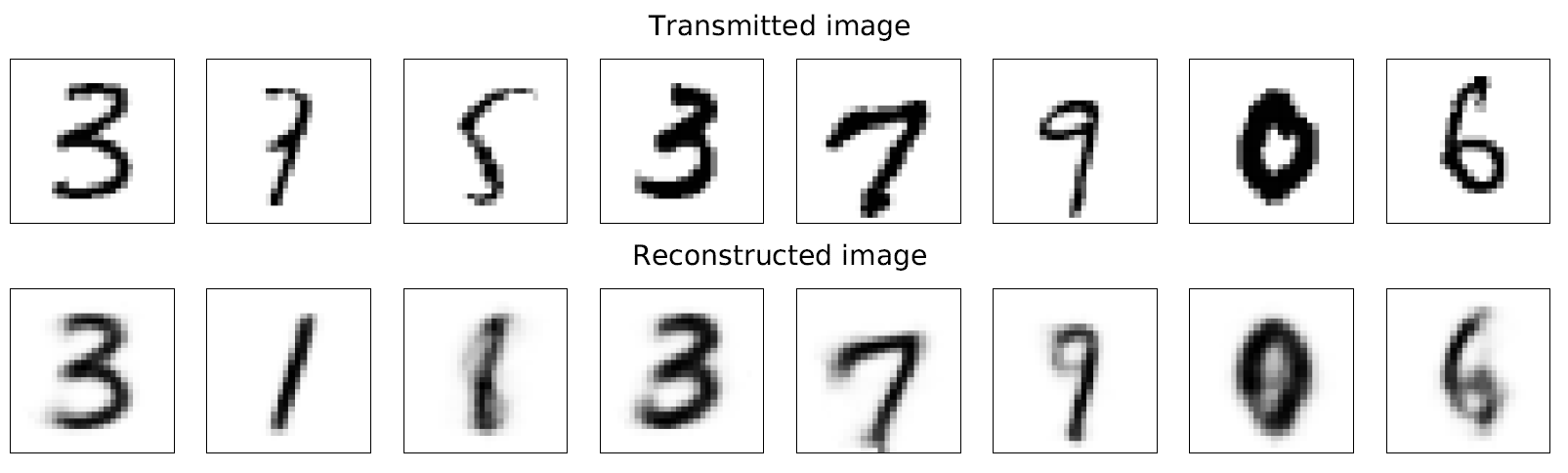
We also consider advanced communication concepts, e.g., the transmission of images with learned joint source and channel coding. The following example shows images (of numbers) that are agressively compressed into a sequence of 24 bits, transmitted over a noisy channel and reconstructed. We can see that despite the noisy transmission, the reconstructed images can be well distinguished:

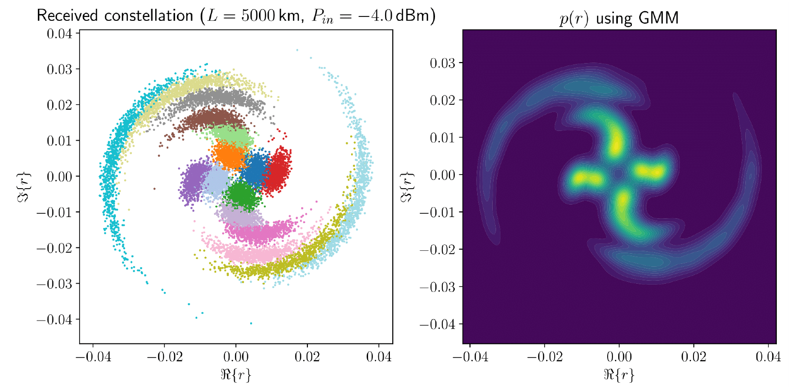
We also investigate advanced detectors, e.g., MIMO detectors, equalizers, etc. We also use machine learning to derive methods for estimating channel parameters like the mutual information of the channel. For this, we use classical density estimators to approximate the probabilistic channel. The following image shows how we can use data from a transmission experiment to approximate the channel using so-called Gaussian mixture models:

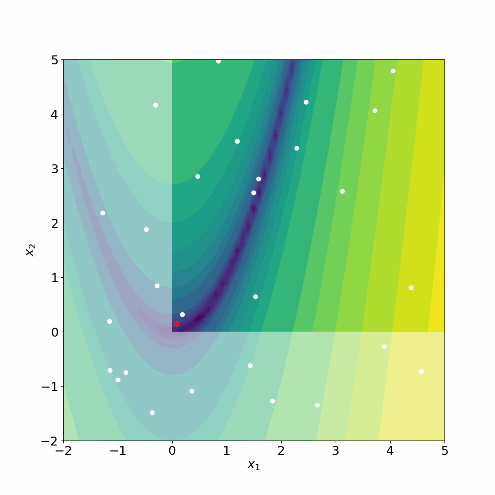
Finally, we also look at scenarios when machine learning methods are not applicable and present optimization methods that do not rely on gradient descent. An example of such an algorithm is differential evoluation, which uses concepts from evolution theory and genetics to find solutions of an engineering problem. The following animation illustrates how this method can be used to find a minimum of a complicated function with constraints. The admissible region is the non-shaded region and the minimum is indicated by the red dot (the true minimum being at (1,1)):

The lecture is accompanied by a tutorial and by a programming competition, where the participants can solve a communication engineering related problem and present their solution. The successful participants of the competition will receive a bonus in the exam.